Heat Transfer Unveiled A Comprehensive Guide to Thermal Energy
Welcome back to MyExamRevision! In today’s blog post, we’re diving into the fascinating world of heat transfer. When objects are heated, energy flows and is stored in their thermal energy reserves. Let’s explore the three methods through which heat can be transferred and the unique ways they impact different materials and environments.
If you’re looking for a tailored and comprehensive approach to understanding heat transfer dynamics – conduction, convection, and radiation – your search ends here. My personalized tutoring is designed to cater to your unique learning style, pace, and academic goals. Together, we’ll unravel the complexities of energy movement and excel in grasping this fundamental concept.
Whether you’re preparing for your upcoming studies or seeking to deepen your knowledge, take the next step by clicking this link:Physics Private Tutoring
Unlocking the Mysteries of Gravity, Weight, and Energy delves deep into the fascinating realm of physics, offering insights into fundamental principles. Explore this captivating topic now:Unlocking the Mysteries of Gravity, Weight, and Energy
Contents
Chapter 1
Conduction: Vibrational Energy Transmission
Chapter 2
Thermal Conductivity: Efficiency of Conduction
Chapter 3
Convection: Fluid Dynamics of Heat Transfer
Chapter 4
Radiation: The Silent Traveler of Heat
Chapter 5
Conclusion: Unraveling the Tapestry of Heat Transfer
Chapter 1
Conduction: Vibrational Energy Transmission
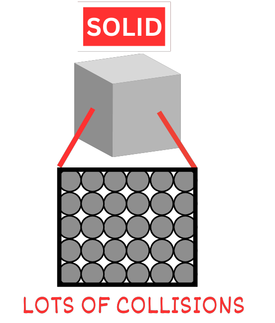
Let’s start our exploration with conduction, a heat transfer mechanism that primarily occurs in solids. The underlying principle here revolves around the vibrating particles within a substance, which transfers energy to their neighbouring particles through these vibrations.
Imagine heating one end of a metal rod. As the energy is supplied, it’s absorbed by the particles at that end, intensifying their kinetic energy and causing them to vibrate more vigorously. These high-energy particles then collide with adjacent particles, transmitting their energy in a chain reaction. This transfer of kinetic energy continues throughout the substance until a state of equilibrium is achieved, resulting in uniform temperature distribution.
Conduction is especially effective in solids due to the close proximity of particles. The tightly packed structure allows for efficient energy transmission through frequent collisions and interactions. In contrast, liquids and gases have particles that are more spaced out, making conduction less efficient in these mediums.
Chapter 2
Thermal Conductivity: Efficiency of Conduction
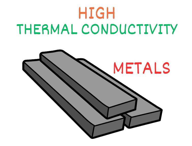
The efficiency of conduction is quantified by a property known as thermal conductivity. Metals, characterized by their closely packed atomic arrangements, exhibit high thermal conductivity.
Consequently, metals can rapidly transfer heat energy over relatively large distances. This property is harnessed in various applications, from cooking utensils to heat sinks in electronics.
On the other hand, substances with lower thermal conductivity, such as plastics, serve as effective insulators. This is why plastic handles on cooking utensils stay cooler even when the metal part is heated. The ability to control heat transfer by exploiting thermal conductivity variations is essential in engineering and design.
Chapter 3
Convection: Fluid Dynamics of Heat Transfer
Convection takes center stage when we shift our focus to fluids, encompassing both liquids and gases. Unlike solids, the particles in fluids are not fixed in place; they can move freely.
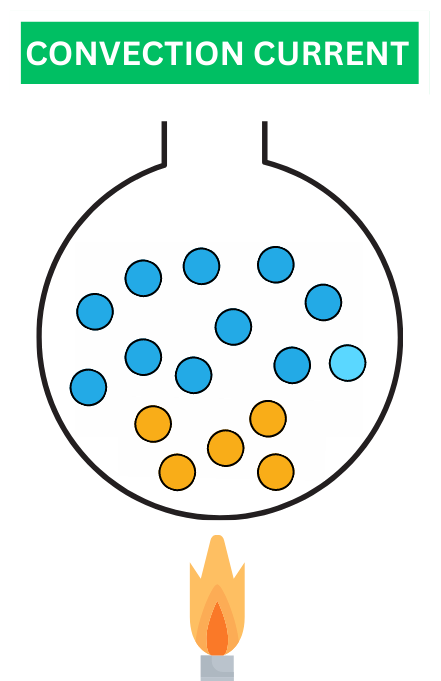
When a fluid is heated, its particles gain kinetic energy, leading to increased motion and random diffusion. This phenomenon causes the more energetic particles to move away from the heat source and towards cooler regions.
As the warmer fluid rises due to its reduced density, it creates an upward flow. Conversely, the cooler, denser fluid near the heat source descends. This circulation of fluid due to temperature differences is referred to as a convection current. You might have witnessed convection currents in action when observing a pot of water heating on a stove. The warmer water near the bottom rises, while cooler water descends to take its place. This movement contributes to the even distribution of temperature within the fluid.
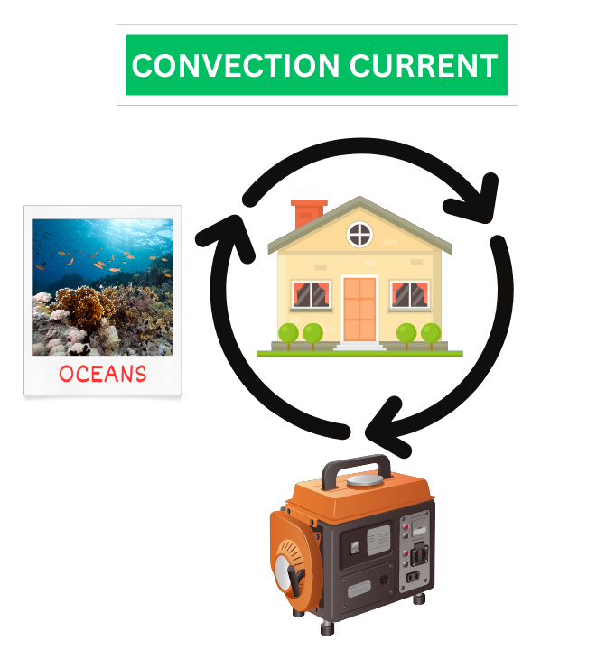
Convection currents are not limited to kitchen scenarios – they play a crucial role in various natural phenomena. For instance, ocean currents are driven by convection currents, which in turn influence climate patterns around the world.
Chapter 4
Radiation: The Silent Traveler of Heat
While conduction and convection rely on particles for heat transfer, radiation offers an entirely different mechanism. In contrast to the first two methods, radiation doesn’t require a medium or particles to propagate. It can occur even in the vacuum of space. This makes radiation a vital player in the universe’s energy balance.
Radiation occurs through electromagnetic waves, specifically in the infrared region of the electromagnetic spectrum. All objects with a temperature above absolute zero emit radiation. The amount of radiation emitted by an object is directly related to its temperature – hotter objects emit more radiation.
You may have experienced this phenomenon firsthand when standing near a barbecue grill. Even if you’re not touching the grill, you can feel the heat radiating from it.
Radiation is an integral aspect of Earth’s energy budget. The Sun’s energy, radiated as electromagnetic waves, reaches our planet and is absorbed by the surface. The surface then re-emits this energy as lower-energy infrared radiation, contributing to Earth’s overall heat balance.
Chapter 5
Conclusion: Unraveling the Tapestry of Heat Transfer
And there you have it – a comprehensive journey through the intricate world of heat transfer. From the vibrating particles in solids to the fluid dynamics of convection and the silent journey of radiation, these mechanisms shape our understanding of energy exchange. Each method, governed by unique principles, offers insights into the behaviour of heat energy in various scenarios
As you go about your daily life, remember that the transfer of heat energy is at the heart of countless natural processes, technological innovations, and environmental phenomena. We hope this exploration has deepened your appreciation for the multifaceted nature of heat transfer. Until our next adventure, stay curious and keep exploring the wonders of the physical world!
SUVAT Equations: Master All Formulas for A Level Kinematics
This is your complete guide to mastering all the SUVAT Equations and their applications in A-Level Kinematics.
If you’re looking to excel in A-Level Mechanics
then You are at the right place.
If you’re seeking a more personalized and tailored approach to mastering SUVAT Equations, look no further. My one-to-one tutoring is designed to cater to your unique learning style, pace, and academic goals.
Whether you’re preparing for your GCSE or A-Level exams, you can click on this link: Physics Private Tutoring
Uncover further insights into the fascinating realm of Variable Acceleration by simply clicking on the link provided for an in-depth exploration: Variable Acceleration
Contents
Chapter 1
All SUVAT Equations
Chapter 2
Deriving SUVAT Equations
Chapter 3
SUVAT in 1D Motion
Chapter 4
Applications of SUVAT Equations
Chapter 5
SUVAT Equations for Variable Acceleration
Chapter 1
All SUVAT Equations: Their Formulas and Meaning of all Symbols
In this chapter, we will explore all the essential SUVAT Equations,
I’ll show you all their formulas, and the meanings behind each symbol.
Let’s get started
What are SUVAT Equations?
The SUVAT Equations, also known as the kinematic equations, is a set of formulas describing objects’ motion under constant acceleration.
PLEASE REMEMBER: They ONLY Work for Constant Acceleration
Here are the five SUVAT Equations
Final Velocity (v) Formula: v = u + at
Displacement (s) Formula (Alternative): s = (v + u) / 2 * t
Displacement (s) Formula with initial velocity: s = ut + (1/2)at2
Displacement (s) Formula with Final Velocity: s = vt – (1/2)at2
Final Velocity (v) Formula (Alternative): v2 = u2 + 2as
These formulas provide a comprehensive understanding of the relationships between displacement, initial velocity, final velocity, acceleration, and time in kinematic scenarios involving constant acceleration.
Lets try to use this formulas in coming chapters.
But if you want a calculator to simply answer all your questions you can simply use this link: Kinematics Questions Calculator
Chapter 2
Deriving SUVAT Equations
Before we dive into the practical applications and start solving Past Paper Questions, it is important to grasp how these equations are derived.
By exploring the derivation process, you will gain valuable insights into the fundamental concepts that govern the relationships between displacement, velocity, acceleration, and time.
So lets see how these equations are derived:
Derivation of the Equation : v = u + at
(Step #1: Start with the formula for acceleration)
a = (v – u) / t
(Step #2: Multiply both sides of the equation by t)
at = v – u
(Step #3: Add u to both sides of the equation)
at + u = v – u + u
at + u = v
Rearrange the equation to obtain the desired form:
v = u + at
Derivation of the Equation : s = (v + u) * t / 2
(Step #1: Start with the formula for average Velocity)
v_avg = s / t
(Step #2: Plug in the formula of v_avg)
v_avg = (v + u)/2
(v + u)/2 = s / t
(Step #3: Multiply “t” on both sides)
(v + u)*t/2 = s
Rearrange the equation to obtain the desired form:
s = (v + u)*t/2
Derivation of the Equation : s = ut + (1/2)at2
(Step #1: Start with the formula for displacement found previously)
s = (v + u)*t/2
(Step #2: Substitute the final velocity formula: v = u + at)
s = (u + at + u)*t/2
(Step #3: Simplifying)
s = (2u + at)*t/2
Rearrange the equation to obtain the desired form:
s = ut + (1/2)at2
Derivation of the Equation : s = vt - (1/2)at2
(Step #1: Start with the formula for displacement formula we got earlier)
s = ut + (1/2)at2
(Step #2: Plug in the formula of v = u + at)
v = u + at
v – at = u
s = (v – at) t + (1/2)at2
(Step #3: Simplify)
s = vt – at2 + (1/2)at2
s = vt – (1/2)at2
Derivation of the Equation : v2 = u2 + 2as
(Step #1: Start with the formula for acceleration)
a = (v – u) / t
at = (v – u)
t = (v – u) / a
(Step #2: Write the formula of s)
s = (v + u)*t/2
(Step #3: Substitute “t”)
s = (v + u)*(v – u) / 2a
(Step #4: Simplifying)
2as = (v + u)*(v – u)
2as = v2 – u2
Rearrange the equation to obtain the desired form:
2as + u2 = v2
v2 = u2 + 2as
Chapter 3
SUVAT in 1-D Motion
1D, or one-dimensional motion, refers to the movement of objects in a single direction or a straight line.
The SUVAT equations we have learned are specifically designed for 1D motion scenarios. This means that the displacement, initial and final velocity, and acceleration all occur in a single direction.
It is essential to keep this in mind whenever you apply any of these equations.
Steps to Solve Problems Involving SUVAT
Step 1: Sketch a Diagram
Begin by sketching the given situation or enhancing the existing diagram provided in the problem.
Incorporate all relevant values and key information from the question.
It is crucial to clearly indicate the one direction as positive and the other as negative.
For Eg: If you have a vertical motion and you choose the UP direction as Positive, then DOWN will be negative
Or
If you have a horizontal motion and you choose the RIGHT direction as Positive, then LEFT will be negative
Step 2 : Identify Knowns and Unknowns
Note down what you already know and what you are trying to find.
In most cases, you will have knowledge of three variables and aim to determine the fourth.
It is helpful to review each letter in the acronym SUVAT and mark down the variables you know, as well as the one you are attempting to find.
Step 3 : Select the Appropriate Equation(s)
Referencing the knowns and unknowns, choose the SUVAT equation(s) that best fit the problem at hand.
Consider the specific variables involved and select the equation(s) that allow for solving the unknown variable.
Step 4 : Solve the Equation(s)
Proceed to solve the selected equation(s) using the known values and algebraic manipulation.
Ensure that your answer includes the appropriate units and, if applicable, provide the answer in context with the problem statement.
By following these steps, you can effectively tackle problems involving SUVAT equations, allowing you to solve for the desired variables and obtain accurate results.
Now lets look at a Solved Example:
Solved Example : A car accelerates from rest at a rate of 2 m/s2 for a time of 5 seconds. What is the final velocity of the car?
Solution
Step 1 & 2 : Sketch a Diagram & Identify Knowns and Unknowns
Step 3: Select the Appropriate Equation(s)
We need an equation that relates the knowns (u, a, t) to the unknown (v). In this case, we can use the equation:
v = u + at
Step 4: Solve the Equation(s)
Plug in the known values into the equation:
v = 0 + 2 * 5
Simplify and solve:
v = 10 m/s
Answer: The final velocity of the car is 10 m/s.
By following these steps and using the appropriate SUVAT equation, we were able to solve the problem and determine the final velocity of the car.
See How easy it was
Chapter 4
Applications of SUVAT Equations
If you genuinely desire a comprehensive understanding of these equations and their applications, you must develop the ability to determine any unknown variables when given known variables.
But you may be wondering, how exactly do we accomplish this?
Read this chapter to find out.
Application 1: Finding the Displacement of an Object
Solved Example : Suppose an object starts from rest and experiences a constant acceleration of 2 m/s2 for a time interval of 4 seconds.
We want to determine the displacement of the object during this time.
Solution
Step 1 & 2 : Sketch a Diagram & Identify Knowns and Unknowns
Step 3: Select the Appropriate Equation(s)
We need an equation that relates the knowns (u, a, t) to the unknown (s). In this case, we can use the equation:
s = ut + (1/2)at2
Step 4: Solve the Equation(s)
Plug in the known values into the equation:
s = 0(4) + (1/2)(2)(4)2
Simplify and solve:
s = 0 + 16 m
s = 16 m
Answer: Therefore, the object has a displacement of 16 meters during the given time interval.
Application 2: Finding the Final Velocity (v) of an Object
Solved Example : Let’s consider a scenario where an object starts with an initial velocity of 5 m/s and experiences a constant acceleration of 3 m/s2 for a duration of 2 seconds.
Our goal is to determine the final velocity of the object at the end of this time interval.
Solution
Step 1 & 2 : Sketch a Diagram & Identify Knowns and Unknowns
Step 3: Select the Appropriate Equation(s)
We need an equation that relates the knowns (u, a, t) to the unknown (v). In this case, we can use the equation:
v = u + at
Step 4: Solve the Equation(s)
Plug in the known values into the equation:
v = 5 + (3)(2)
Simplify and solve:
v = 5 + 6 m/s
v = 11 m/s
Therefore, the object reaches a final velocity of 11 m/s at the end of the given time interval.
Application 3: Finding the Initial Velocity (u) of an Object
Solved Example: Consider a scenario where an object undergoes uniform deceleration and comes to rest after traveling a distance of 100 meters. The object’s final velocity is 0 m/s, and the deceleration is known to be -2 m/s2. Our goal is to determine the initial velocity of the object.
Solution
Step 1 & 2 : Sketch a Diagram & Identify Knowns and Unknowns
Step 3: Select the Appropriate Equation(s)
We need an equation that relates the knowns (s, a, v) to the unknown (u). In this case, we can use the equation:
v2 = u2 + 2as
Step 4: Solve the Equation(s)
Plug in the known values into the equation:
(0)2 = u2 + 2(-2)100
Simplify and solve:
400 = u2
u = 20 m/s
Application 4: Finding the Time (t)
Solved Example: Let’s consider a scenario where a ball is thrown vertically upward with an initial velocity of 20 m/s. The ball reaches its maximum height and falls back to the ground, ultimately ending at the same point from where it was thrown.
We want to determine the total time of flight, which includes both the upward and downward motion of the ball.
Solution
Step 1 & 2 : Sketch a Diagram & Identify Knowns and Unknowns
Step 3: Select the Appropriate Equation(s)
We need an equation that relates the knowns (s, a, s) to the unknown (t). In this case, we can use the equation:
s = ut + (1/2)at2
Step 4: Solve the Equation(s)
Plug in the known values into the equation:
0 = 20t + (1/2)(-9.8)t2
Simplify and solve:
0 = 20t -4.9t2
t = 0 & 20/4.9
t = 0 & 4.08 s
Since the initial time t = 0 is when the ball was thrown, we disregard this value. Therefore, the total time of flight for the ball is approximately 4.08 seconds.
Chapter 5
SUVAT Equations for Variable Acceleration
In the previous chapters, we explored the applications of SUVAT equations in scenarios with constant acceleration.
However, real-world situations often involve variable acceleration, where the rate of change in velocity varies throughout the motion.
The SUVAT equations with small changes can be used for motion in Variable acceleration as well.
Let’s see How:
SUVAT Equations to Solve Questions for Variable Acceleration
Before we dive into practical examples, let’s familiarize ourselves with the five SUVAT equations in their integration form:
PLEASE REMEMBER: They Work for both Constant and variable Acceleration
Velocity from acceleration: dv = ∫ a dt
Displacement from velocity: ds = ∫ v dt
Acceleration from velocity: a = dv/dt
Velocity from displacement: v = ds/dt
Velocity – Acceleration equation: ∫ v dv = ∫ a ds
Free-Falling Object with Variable Acceleration
Solved Example: Consider a free-falling object with variable acceleration due to air resistance. Suppose the object starts from rest and its velocity changes with time according to the equation v = 9.8t + 4.9t2, where v is the velocity in m/s and t is the time in seconds.
Find the displacement of the object after 3 seconds.
Solution
Step 1 & 2 : Sketch a Diagram & Identify Knowns and Unknowns
Step 3: Select the Appropriate Equation(s)
We need an equation that relates the knowns (t, v) to the unknown (s). In this case, we can use the equation:
ds = ∫ v dt
Step 4: Solve the Equation(s)
Plug in the known values into the equation:
ds = ∫ (9.8t + 4.9t2 )dt
Integrating the equation, we get:
s = 9.8(t2 /2) + 4.9(t3 /3) + C
Plugging in the limits of t as 3 and 0
s = (9.8(32 /2) + 4.9(33 /3) + C) – (9.8(02 /2) + 4.9(03 /3) + C)
s = 88.2 m
Accelerating Car with Variable Acceleration
Solved Example: Suppose a car starts from rest and accelerates with an acceleration given by a = 2t, where a is the acceleration in m/s2 and t is the time in seconds.
Find the distance traveled by the car after 5 seconds.
Solution
Step 1 & 2 : Sketch a Diagram & Identify Knowns and Unknowns
Step 3: Select the Appropriate Equation(s)
We need an equation that relates the knowns (t, a) to the unknown (s). In this case, we can use the equations:
dv = ∫ a dt
ds = ∫ v dt
Step 4: Solve the Equation(s)
Plug in the known values into the equation:
dv = ∫ (2t) dt
Integrating the equation, we get:
v = t2 + C
Now since the initial velocity is Zero, so at t = 0, v = 0
0 = 02 + C
we get C = 0
v = t2
ds = ∫ v dt
ds = ∫ t2 dt
s = t3 / 3 + C
Again here, since the initial velocity is Zero, so at t = 0, s = 0
0 = 03 + C
again, we get C = 0
s = t3 / 3
At t = 5 sec
s = 53 / 3
s = 41.67 m
These examples demonstrate how to apply the integration forms of SUVAT equations for variable acceleration to solve practical motion problems.
By understanding and utilizing these equations, you can analyze and predict the behavior of objects in motion with changing acceleration
If you’ve enjoyed diving into the world of SUVAT Equations and want to take your understanding to the next level, consider joining my one-to-one private tutoring sessions.